What is Risk?

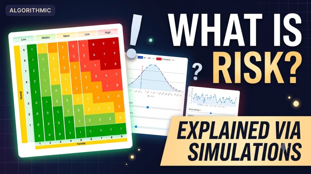
Risk is the possibility of an unfavorable event occurring. Mathematically and conceptually, it is driven by two distinct variables: probability (the likelihood or uncertainty of the event) and impact (the scale of the consequence). If either of these variables is zero – meaning there is absolute certainty about the outcome, or the outcome has zero consequence – then risk does not exist.

Risk = Probability x Impact x Exposure

Exposure refers to actual part of impact you are exposed to. If you own a building and you have insured it for natural desasters. In an event where you loose the entire building, impact is 100% but due to insurance your expose is very little. When exposure is not mentioned in the formula, it is considered part of the impact. Therefore mostly Risk = Probability x Impact is used omitting the exposure.

Both exposure and impact are based on current data, but probability is often calculated based on past data. That why this is the most important part of the equation. To calculate the probability, difference statistical models are used. Now a days AI/ML is being employed more and more to accurately predict the probability.

While we often think of risk exclusively as a negative event – like losing money or suffering an injury – in professional and mathematical terms, risk simply represents the deviation from an expected/targeted outcome. That is why risk is measured using standard deviation which means how spread out numbers are from their average (mean).

Same thing is presented professionaly using bell curve. A risk bell curve (normal distribution) is a visual graph where moderate outcomes cluster in the middle (the peak), while rare, extreme outcomes – both good and bad – taper off into flat “tails” on either side. It shows that standard, average risks are highly predictable, while true catastrophes or windfalls are very unlikely to happen.

While a symmetrical bell curve is a great starting point, real-world markets rarely behave so neatly. In practice, risk analysts must look out for two major deviations:

• Skewness (Asymmetry): A standard bell curve is perfectly balanced, but real-world returns are often tilted to one side. In finance, we often see negative skewness – where an asset enjoys small, steady gains most of the time, but is prone to sudden, massive drops (like picking up pennies in front of a steamroller).
• Fat Tails (Extreme Events): In a theoretical bell curve, extreme events (the thin “tails” on the far left and right) are mathematically next to impossible. In reality, market crashes, political shocks, and black swan events happen far more frequently than a standard curve predicts. Because these tails are “fatter” than expected, relying strictly on a perfect bell curve can leave you dangerously underprepared for catastrophic losses.

When making practical financial decisions, we typically look at the average return (the expected value) as our baseline. For example, if you evaluate an investment opportunity with an average projected return of 12%, and your total cost of capital is 10%, the positive spread of 2% makes the investment viable on paper.

However, the average return only tells half the story. Consider three distinct investment opportunities, all sharing the same 12% average return:

1. 12% flat return.
2. Lowest return is 10% and highest is 14%
3. Lowest is 6% and highest is 18%.

Which one will you take?

The option one represents a guaranteed, consistent return with zero variance. It is the safest option. Option two has low volatility. The returns are clustered very tightly around the 12% average, meaning you are highly likely to get a result very close to your expected outcome. Option three represents higher volatility (risk). While the average is still 12%, the outcomes are more spread out. You have the potential for higher gains (up to 18%) but also the risk of lower returns (down to 6%).

The “right” choice depends entirely on your personal investment philosophy and financial goals. You will choose option one if you are risk-averse. You prioritize predictability and capital preservation above all else, and you are satisfied with a guaranteed 12% without the possibility of underperforming. Option two is for you, if you are conservative-to-moderate. You are comfortable with a very small amount of fluctuation in exchange for the high probability that your final return will be very close to 12%. But if you are a risk-seeker and you are willing to endure higher uncertainty and lower-than-average returns in specific scenarios because you want to “maximize” the potential for higher upside (18%), option three is for you.

To see this concept in action, we can look at the real-world performance differences between Treasury Bills (T-Bills)—which represent a guaranteed, risk-free government security similar to Opportunity 1—and First IBL Modaraba (FIBLM) on the Pakistan Stock Exchange (PSX) during the first half of 2026 (1st Jan 2026 to 30th Jun 2026):

1. Government Treasury Bills: Provided a highly secure, predictable, and flat yield with near-zero volatility, shielding investors from market downturns.
2. FIBLM (First IBL Modaraba): Exhibited significant equity market volatility, trading in a wide 52-week range of Rs. 5.00 to Rs. 22.24. This asset offered the possibility of massive, market-beating returns, but exposed investors to the downside risk of capital erosion during market corrections.

If you want to avoid risk, you will probably choose investment in treasury bills, however if you want higher returns and accept the risks associated, you will choose FIBLM.

Time is also plays significent role in risk. Some risks increase over time, while some risk decrease in the long run.

1. Long-term structural uncertainty increases ($+$ Risk): The farther out you go, the more the “cone of uncertainty” widens. Macro conditions change, new technologies disrupt industries, and unexpected events compound. The absolute range of outcomes gets wider.
2. Short-term noise averages out over time ($-$ Risk): If you measure risk as annualized volatility (the average bumpiness you experience per year), a longer holding period actually smooths out the short-term noise. If you hold an asset for 1 day, your return is highly uncertain. If you hold it for 20 years, the short-term ups and downs cancel each other out, giving you a much more stable, predictable average annualized return.

The Stock Market Example:

• If you invest in the stock market for 1 day, your risk of losing money is nearly 50% because of short-term noise.
• If you invest for 20 years, your annualized volatility is incredibly low, and your risk of a negative annualized return drops close to 0% because the short-term noise averages out (Longer Period = More Certainty).
• However, the absolute dollar amount in your account at Year 20 is much harder to predict than it is for tomorrow. You might end up with $500,000 or $1,500,000 depending on the decades-long economic cycle (Longer Period = More Cumulative Uncertainty).

This is called diversification strategy, which is based on the principle that holding risky assets, like stocks, over longer periods can lower the risk of annualized losses. Because negative returns tend to be offset by positive ones over extended horizons, financial planners often suggest younger investors take on more equity risk.

However, this is traditional view. In the the academic view, nobel laureates like Paul Samuelson and Zvi Bodie have argued that time diversification is a mathematical fallacy. While your annualized volatility drops, the total potential magnitude of loss (due to compounding) grows larger over time. Furthermore, if investment returns are independent from year to year, risk does not inherently diminish simply because of the passage of time.

There are different types of risks. Some of them are mentioned below. We will discuss these in their respective topic.